
Service Robot Downtime Cost & OEE — Measuring What Idle Machine Hours Actually Cost
At a glance: Manufacturing has measured asset effectiveness for decades; autonomous cleaning fleets mostly have not. This guide adapts the OEE triangle to service robots, ranks the four downtime categories by their real cost, and works a three-unit fleet through to a USD 70,500 annual figure — including why 100% availability is the wrong target.
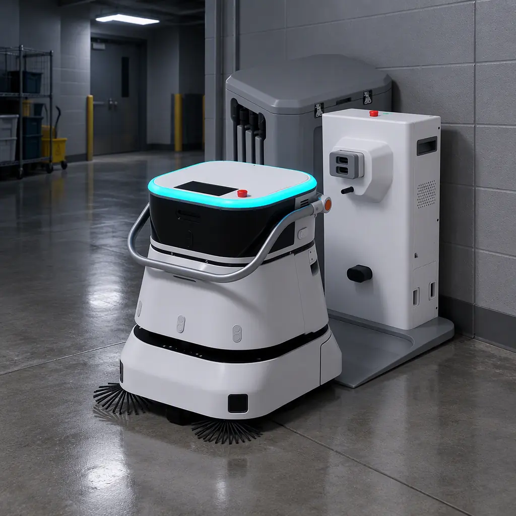
Manufacturing has measured asset effectiveness for forty years. A production line that runs 80% of scheduled hours is understood, benchmarked and managed. A robot fleet that runs 68% of scheduled hours is usually not measured at all — the site knows the machines exist, knows someone services them, and has no number for what the idle hours cost. This guide builds that number, using the same OEE structure manufacturing already trusts.
The gap matters because robot downtime is not like staffing absence. If a cleaner calls in sick, the shift is short-staffed and some floor goes unwashed. If a scrubber is down for four days awaiting a part, the same floor goes unwashed, and the operation has also paid for a capital asset that produced nothing for four days. The second cost is invisible unless it is modelled.
Adapting OEE to a Service Robot Fleet
OEE in manufacturing is availability × performance × quality. The translation to service robots is direct once each term is defined in cleaning terms rather than production terms.
| OEE Term | Manufacturing Meaning | Service Robot Meaning | Typical Figure |
|---|---|---|---|
| Availability | Run time ÷ planned production time | Scheduled cleaning hours actually delivered ÷ hours the fleet was rostered to clean | 70–85% mature fleets |
| Performance | Actual output ÷ theoretical maximum | Effective m²/h ÷ nameplate m²/h, after obstacles, traffic and route density | 55–75% |
| Quality | Good units ÷ total units | Area passing inspection on first pass ÷ area cleaned, plus rework passes | 80–92% |
Multiplying those three gives an effectiveness figure that is almost always far below what anyone estimated informally. A fleet at 78% availability, 65% performance and 88% quality has an OEE of 44.6%. That is not a failure — it is normal for a first-generation autonomous fleet, and it is exactly why the payback models discussed elsewhere in this series must use an availability factor rather than nameplate output.
The reason to measure all three rather than availability alone is that they have entirely different fixes. Availability problems are service and logistics problems. Performance problems are usually mapping, route or traffic problems. Quality problems are usually consumable, water or scheduling problems. A site that tracks only "is it running" will spend money on the wrong one.
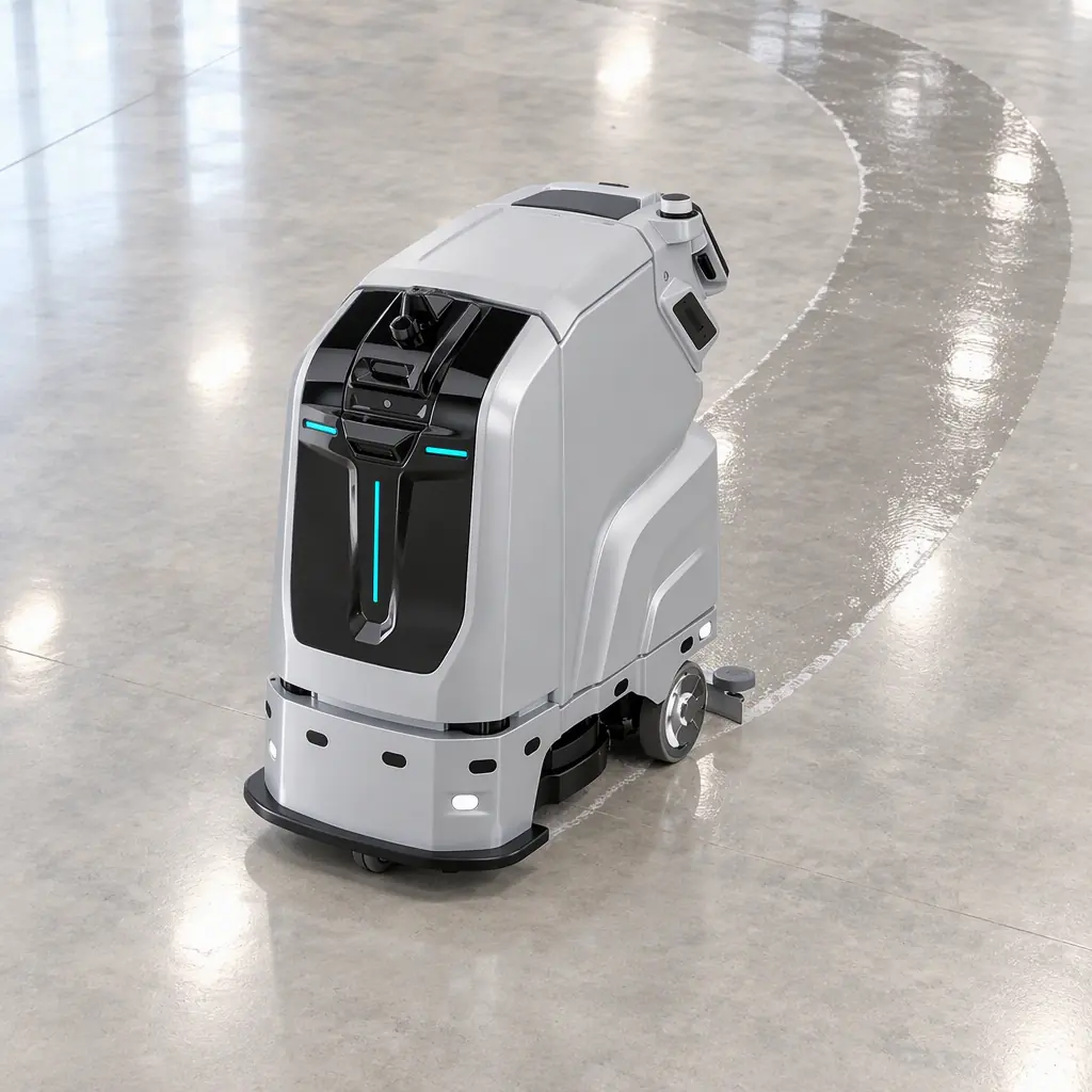
The Four Downtime Categories, Ranked by Cost
Downtime is not one thing. Four categories account for nearly all lost machine hours, and they are not equally expensive because they do not require the same response.
| Category | Typical Share of Lost Hours | Cost Character | Fix |
|---|---|---|---|
| Routine servicing | 25–35% | Planned, absorbed into schedule | Correct — this is not a failure. Move servicing into low-demand windows |
| Consumable and tank cycles | 20–30% | Predictable, proportional to area | Right-size tanks and docks; site water points to cut travel time |
| Interventions and stuck events | 15–25% | Unpredictable, high staff attention cost | Map maintenance, obstacle removal, route redesign |
| Unscheduled repairs and parts waits | 10–20% | Highest cost per hour — asset idle plus substitute labour | Spares strategy, service SLA, regional parts stock |
The first two categories are engineering facts and belong in the productivity model. The second two are the ones worth managing actively, because they are the only ones that also require substitute labour.
Worked Downtime Cost: A Three-Unit Grocery Fleet
Take a supermarket group running three compact cleaning units across two stores, each rostered for a single 7-hour overnight window, 360 operating days a year.
| Line | Value | Derivation |
|---|---|---|
| Rostered machine hours per year | 7,560 h | 3 units × 7 h × 360 days |
| Measured availability | 74% | Available in fleet telemetry |
| Lost hours per year | 1,966 h | 7,560 × 26% |
| Substitute labour rate | USD 21/h | Overnight contract rate, fully loaded |
| Substitute labour cost | USD 41,300/yr | 1,966 × 21 |
| Asset idle cost | USD 12,400/yr | Annualised capital × 26% of the year |
| Service and parts | USD 16,800/yr | Contract plus unscheduled repairs |
| Total downtime cost | USD 70,500/yr | Sum of the three lines |
Two conclusions follow. First, the substitute labour line is the largest single component, and it scales with the labour rate rather than with the machine — a supermarket in a high-wage market will see a materially worse figure for the same 26% availability gap. Second, moving availability from 74% to 84% removes roughly USD 27,000 of that total, which is typically more than any single hardware upgrade in the same period would deliver.
Do Not Aim for 100% Availability
The instinct on seeing a 26% availability gap is to close all of it. That is the wrong target, and pursuing it wastes money.
Some availability loss is structural and beneficial. When a machine stops to drain and refill, it is protecting its recovery system from running dry and damaging brushes. When it returns to dock at a planned threshold, it is extending battery life. When it is excluded from a busy trading window, it is reducing safety exposure with customers present. A fleet driven to 95% availability by suppressing these stops would have higher consumable costs, shorter asset life and a worse safety record.
The realistic target is a bounded range, and the right range depends on the building. A closed industrial site can run higher availability than a retail environment with unpredictable public traffic. What matters is not the number itself but whether the lost hours are known, categorised and costed. A site that knows its 26% gap is 30% servicing, 26% tank cycles, 22% interventions and 22% repairs (by hours) can act on the bottom two and accept the top two.
The Operational Levers That Actually Move Availability
Five interventions deliver most of the available improvement, in rough order of return on effort.
| Lever | Expected Availability Gain | Why It Works |
|---|---|---|
| Map maintenance discipline | 3–6 points | Most intervention events trace to a changed obstacle or a stale map. A recurring re-mapping routine removes the largest single cause |
| Remote diagnosis and OTA updates | 2–4 points | Many faults are resolved without dispatching an engineer, cutting the time between fault detection and fix |
| On-site consumable stockholding | 2–3 points | Brush, squeegee and pad replacement happens within the shift instead of at the next delivery |
| Regional spares strategy | 3–5 points in repair events | Directly attacks the parts-wait category, which carries the highest cost per lost hour |
| Dock and infrastructure siting | 1–3 points | Docks placed where the machine works rather than where the power was available cuts travel and turnaround time |
The spares lever deserves emphasis because it is the one procurement teams most often price out of a deal. Contractual service levels without regional parts stock produce a guarantee that a technician will be dispatched, which is not the same as a guarantee that the machine will be repaired. The distinction is set out in the service-level section of the maintenance and TCO guide, and the supply-chain side of the same question is covered in the vendor evaluation framework.
Instrumenting the Fleet So the Number Exists
Downtime modelling fails at most sites for one reason: the data was never captured. Fleets that report only task completion cannot distinguish between a machine that stopped and a machine that was never scheduled.
Four data points are sufficient to run the model, and modern fleet platforms capture all four natively as described in the custodial fleet management software guide.
- Scheduled versus delivered cleaning hours per unit per shift — the availability input. Without this the whole calculation is guesswork.
- Effective area per delivered hour — the performance input, and the only honest way to compare your site against a nameplate rate.
- Stop events with reason codes — separates a tank cycle from a fault. A fleet that logs stops without categorising them cannot be optimised.
- First-pass inspection results — the quality input, and the single most commonly missing measure in service robot reporting.
With those four streams the OEE figure becomes a monthly management number rather than an annual post-mortem. It also becomes the basis for the fleet utilisation analysis that decides whether the site needs more machines or better machines — the same question addressed from the sizing side in the fleet charging infrastructure guide.
Send us your rostered hours, current availability and the split of lost time by cause, and we will build your downtime cost model alongside the OEE triangle, so the improvement case is quantified before any capital is committed. Contact us.