
Fleet Charging Infrastructure — Power Planning for a 20-Robot Deployment
At a glance: Charging infrastructure is where robot capital projects lose their schedule. The machines arrive in weeks; the electrical work has a permit queue. This guide works through the load arithmetic for a 20-unit fleet from first principles, the dock layouts the AOMAN C1 physically requires, why a demand charge — not energy cost — dominates the operating economics, and how to sequence installation so the fleet arrives to live docks instead of extension leads.
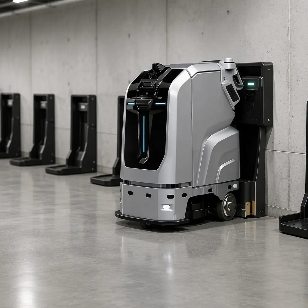
Every robot fleet deployment has two schedules: the machine schedule and the electrical schedule, and they are almost never the same length. Robots can be specified, manufactured and delivered in six to ten weeks. A new electrical panel with conduit runs, breaker additions, floor cores and a certificate of compliance runs on the electrician's queue, the permit queue and the building's change-control process. When a deployment slips, it is nearly always because the second schedule was treated as a detail of the first.
This guide treats charging as an infrastructure project with a lead time, because that is what it is. The arithmetic below is built from published AOMAN hardware specifications so a facilities engineer can audit every number.
Step 1: Establishing the Per-Unit Load
Charging load is not the same as the charger's nameplate rating, and starting from the robot rather than the dock keeps the estimate honest. The AOMAN C1 carries a 24 V / 120 Ah lead-acid pack with roughly 8 hours to full charge, a configuration compared against LFP and LTO alternatives in the battery technology guide. Nominal energy is straightforward: 24 V × 120 Ah = 2,880 Wh, or 2.88 kWh per full cycle.
Divide 2,880 Wh by an 8-hour charge window and the average draw is 360 W per unit. That number is the floor, not the design figure. Charging is not linear — a lead-acid pack accepts higher current in its bulk phase than in absorption — so the instantaneous draw during bulk charge runs meaningfully above the average. Designing to the average understates the branch circuit requirement and produces nuisance breaker trips in the first week.
Design rule. Size branch circuits to the charger's nameplate input current, and size the panel and aggregate load to the average draw multiplied by fleet count with a diversity factor applied. Confusing the two is the most common engineering error in robot charging: one number is a safety requirement, the other is a capacity requirement, and they are not interchangeable.
Step 2: The 20-Unit Fleet Arithmetic
Taking the AOMAN C1 as the reference unit, and using an 8-hour simultaneous charge window as the worst realistic case, the fleet load builds up as follows.
| Quantity | Per Unit | 20 Units | Notes |
|---|---|---|---|
| Battery energy per cycle | 2.88 kWh (24 V × 120 Ah) | 57.6 kWh | Full charge from empty |
| Average charging draw | ~360 W over 8 h | ~7.2 kW | Continuous average across the charge window |
| Bulk-phase peak | Charger nameplate (typically 1.2–1.8× average) | ~9–13 kW | Drives branch circuit sizing, not panel capacity |
| Daily energy consumption | ~2.9 kWh (one cycle) | ~58 kWh/day | Assumes one full cycle per unit per day |
| Monthly energy | ~87 kWh | ~1,740 kWh/month | At one cycle per day, 30 days |
The energy number is the least interesting figure in the table, and that is the point. At typical commercial electricity rates, 1,740 kWh per month is a modest utilities line — the fleet's energy cost is not what threatens the business case. What threatens it is how that energy is drawn and when, which is the subject of the next two sections.
Two refinements matter in practice. First, a fleet does not charge on a single cycle per day. Cleaning robots in multi-shift operations charge opportunistically between windows, and a 16-hour duty cycle can push a unit through 1.5 to 2 partial cycles daily — so daily energy should be modelled against actual duty profile, not a nominal one. Second, the mixed-fleet case changes the arithmetic: a C2 Pro charges in approximately 3 hours rather than 8, so its instantaneous draw is higher even though its total energy per day is comparable. A fleet of twenty mixed units must be sized per unit class, then aggregated.
Step 3: Why the Demand Charge Decides the Economics
Most facilities evaluate robot charging on energy cost per kilowatt-hour and conclude it is negligible. That conclusion is usually right about energy and wrong about the bill, because the dominant cost of an electrical load in a commercial building is frequently the demand charge — a monthly fee based on the highest 15- or 30-minute averaged demand the building places on the grid, not on total consumption.
The mechanism matters because robot charging is unusually concentrated. If a 20-unit fleet docks at 21:00 and begins charging simultaneously, it presents a step change in building load of several kilowatts inside a single billing interval. If that interval happens to coincide with an existing peak — an HVAC morning start, a kitchen lunch service, a production shift start — the fleet does not add its own demand charge so much as worsen a peak that already existed, and the increment persists for the whole billing month.
Three mitigations are available, in ascending order of sophistication.
Staggered start times. The simplest and most effective. Spread dock start times across a 60–90 minute window so the fleet's bulk-charge phase never occurs all at once. No additional hardware; implemented in the scheduling layer. This single measure typically removes the fleet's contribution to the monthly peak demand and costs nothing.
Scheduled charging windows. Move the charging window into the low-tariff period where a time-of-use tariff applies. The AOMAN C1 charges over roughly 8 hours, which is generous enough to shift a whole window rather than merely stagger within it. This captures both tariff and demand benefit, provided the fleet still has enough charged capacity for the next cleaning window — the constraint that binds in multi-shift operations.
BMS-coordinated demand response. Where the building already runs a building management system, the fleet can be registered as a controllable load and throttled or deferred during building peaks. Twenty C1 units at roughly 360 W average represent over 7 kW of controllable load — small against a large building's total demand, but genuinely useful as fast, interruptible capacity precisely because a cleaning cycle can shift by hours with no operational consequence. This is examined as an integration pattern in the BMS integration guide.
Step 4: Dock Siting at Real Machine Dimensions
Dock layout is a physical design problem, and the AOMAN C1 sets the constraints. At 1,210 × 580 × 1,160 mm (H×W×D) and 227–254 kg, it is not a device that can be tucked into a janitor's closet or charged in a corridor. The dock zone needs to be planned as a machine bay, not as an electrical outlet.
| Dock requirement | Specification | Why it is non-negotiable |
|---|---|---|
| Sleeping footprint | 1,210 × 580 mm body, plus approach clearance | Access to the body for tank drain, brush change and squeegee service must remain possible while docked |
| Turning clearance | 200 cm minimum | Auto-docking is an infrared-guided manoeuvre; insufficient clearance turns every dock event into a manual intervention |
| Approach surface | Flat, dry, level access | 6° ramp limit and 5 cm toe-height obstacle sensing; a wet or sloped dock approach defeats auto-docking |
| Water access nearby | Within practical hose range | 120 L total tank capacity (70 L clean / 50 L dirty) means frequent fill and drain cycles |
| Network coverage | Reliable Wi-Fi or cellular at the dock point | Firmware, cleaning logs and fleet coordination all require connectivity where the robot parks; concrete and below-grade areas need remediation |
| Drainage or bunding | Containment for drain-down water | Tank emptying at the dock releases water; a dock without drainage turns a service bay into a slip hazard |
A practical layout for a 20-unit fleet is two to three bays of six to eight units, not one wall of twenty. Splitting the fleet reduces the length of the cable and conduit run, keeps each bay within reach of a water point, and limits blast radius — a fault in one bay's supply does not ground the entire fleet. It also makes phased installation possible, which is the subject of the next section. Where docks span more than one floor or building, the lift interfaces described in the elevator integration guide have to be resolved before the bay plan is finalised.
Step 5: Phased Capex Instead of a Single Hit
Twenty docks provisioned in one electrical project is a large, slow, capital-intensive line item that has to be approved before a single robot is confirmed working. Vehicles and platforms solve this with phased rollouts, and robot fleets can use the same structure.
| Phase | Units | Infrastructure | Purpose |
|---|---|---|---|
| Pilot | 2–4 | 1 bay, 1 circuit group, temporary or leased docks | Validate cleaning performance, dock discipline and operator workflow with minimal electrical work |
| Tranche 1 | 8–10 | 1 permanent bay, new panel with spare breakers | Prove the panel and bay design; size with headroom for tranche 2 |
| Tranche 2 | 20+ | Second bay, conduit runs already rough-fitted in tranche 1 | Scale within an existing electrical design; no new permit cycle |
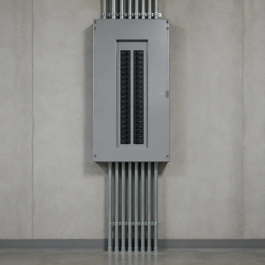
The critical discipline is rough-fitting tranche 2 during tranche 1. Conduit and panel capacity cost little when installed alongside other work and a great deal when added as a standalone change. A panel specified with spare breaker positions and conduit routed to the second bay position turns a future project into a future connection.
Step 6: Sequencing the Project Correctly
Once installation and machine delivery are treated as two schedules, the sequencing question becomes concrete. The order below reflects where deployments actually lose time.
| Order | Activity | Typical Lead Time | Runs In Parallel With |
|---|---|---|---|
| 1 | Site survey: dock zone, panel capacity, conduit route, water and drainage access | 1 week | Fleet specification |
| 2 | Electrical design and load calculation approved | 2–3 weeks | Fleet order placement |
| 3 | Permit application (where required) and electrician scheduling | 3–8 weeks | Robot manufacturing lead time |
| 4 | Conduit, panel and branch circuit installation | 1–3 weeks | Robot shipping |
| 5 | Dock hardware, drainage and network at dock | 1 week | Robot commissioning prep |
| 6 | Commissioning: mapping, dock calibration, first charge cycles | 1–2 weeks | Operator training |
Read down the right-hand column and the strategy is visible: the electrical project should start before — or simultaneously with — the fleet order, and the permit application is the longest pole. A deployment that begins electrical design at the same time it places the robot order arrives at commissioning with live docks; one that begins electrical work when the robots arrive has a two-month idle fleet.
Step 7: What to Verify After Installation
Commissioning is not complete when the first robot charges. Six checks confirm the installation will hold up under fleet load rather than under a single unit's demand.
Measure actual bulk-phase current on one circuit and compare it against the charger nameplate. If measured draw exceeds nameplate, the branch circuit is undersized and will trip as the fleet scales.
Verify the panel has spare capacity for the next tranche without a service upgrade. Record the spare breaker positions and remaining panel capacity in the asset register, not in a commissioning report that will be filed and forgotten.
Test simultaneous dock events. Charge the full pilot fleet at once and observe the main breaker and the building's demand logger. This is the cheapest possible test of the demand-charge strategy and it is routinely skipped.
Confirm auto-docking success rate over twenty consecutive attempts per dock. Below roughly 90% success indicates a clearance, approach-surface or lighting problem at the dock, all of which are solvable and all of which degrade to manual intervention if ignored.
Check network stability at the dock over a full charge cycle. Dock connectivity failures are silent — the robot charges, but logs and firmware updates fail, and the fleet platform shows stale data.
Validate thermal and ventilation conditions in the dock bay. Lead-acid charging releases hydrogen; a sealed, unventilated closet retrofitted as a charging bay is a safety and code problem, not merely a performance one.
The Operational Cost You Will Actually Feel
Returning to where this guide started: the energy bill is not the pain. The three costs that show up in real deployments are dock footprint consumed from service space, the labour cost of manual interventions when auto-docking underperforms, and the cost of charging at the wrong time on a demand-charge tariff.
Of those three, only the third is invisible until the utility bill arrives, and it is the one that a scheduling decision can eliminate at zero capital cost. The planning work that pays is therefore not buying cleverer chargers but understanding the building's load profile well enough to choose when the fleet charges. Where a fleet is being deployed alongside broader energy management, the same controllable-load logic connects to time-of-use tariffs and demand response through the BMS — the pattern described in the battery and charging architecture guide and costed in the maintenance and TCO model.
Send us your dock zone dimensions, the building's main panel capacity and your fleet target — we will help you derive the branch circuit, panel and dock layout figures for your site, and sequence the electrical work so the fleet arrives to live docks. Contact us.