Cleaning Robot Labor Cost Model — The Worked Arithmetic Behind the Savings Claim
At a glance: Every cleaning robot business case rests on four inputs and one output, and the fourth input — machine availability — is the one vendors leave out. This guide builds the model in the open: a 12,000 m² shopping centre worked end to end, the three cost lines between gross and net saving, and the two assumptions that move payback further than machine price ever will.
The two questions facility managers ask first are almost never the questions the industry answers. They ask how much a machine saves per square metre, and when the money comes back. What they get instead is a machine specification sheet and a case study from a building that is nothing like theirs. This guide does the arithmetic properly, in the open, with numbers you can substitute your own rates into.
The method has four inputs and one output. Get the four inputs right and the output is defensible in a budget meeting. Get them wrong — and the most common error is using nameplate cleaning rate as productive output — and the model will be wrong by a factor of two.
The Four Inputs, and Why the Fourth Is Always Wrong
Labour-cost modelling for cleaning automation reduces to four variables, and only the last one is routinely overstated.
| Input | What It Is | Typical Range | Where It Goes Wrong |
|---|---|---|---|
| Cleaned area | Billable floor area actually cleaned per visit, in m² | Site survey | Using gross floor area instead of cleanable area — fixtures, storage and racking typically remove 15–30% |
| Fully loaded labour rate | Hourly cost including wages, on-costs, supervision and equipment | USD 18–38/h in Western markets | Using base wage only. The fully loaded figure is typically 1.35–1.6× base |
| Productive cleaning rate | m² actually cleaned per labour hour, all tasks included | 150–350 m²/h manual | Quoting the best-case continuous figure. Real labour includes travel, setup, refills and interruptions |
| Machine availability | Share of shift hours the machine is actually cleaning | 55–80% | Assuming 100%. Docking, refill, drains, mapping, interventions and traffic all consume time |
The fourth input is where almost every vendor model fails, and it is the one that decides whether the business case is real. A machine rated at 2,040 m²/h does not clean 2,040 m² every hour of the shift. It cleans that rate while moving, at full brush engagement, on clear floor, with tanks that have not run dry.
Worked Example: A 12,000 m² Regional Shopping Centre
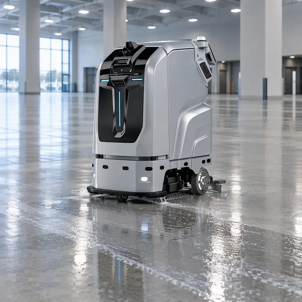
Take a mid-size regional centre with 12,000 m² of cleanable public mall floor, cleaned twice daily. The centre currently runs a night crew of six on a seven-hour productive shift.
| Line | Manual Baseline | Calculation |
|---|---|---|
| Cleanable area per visit | 12,000 m² | Survey figure, fixtures deducted |
| Visits per day | 2 | Day spot-clean, night full scrub |
| Daily cleaning load | 24,000 m² | 12,000 × 2 |
| Manual productive rate | 260 m²/h | Measured, includes refills and travel |
| Labour hours required | 92.3 h/day | 24,000 ÷ 260 |
| Fully loaded labour rate | USD 24/h | Base 16.50 + on-costs + supervision |
| Annual manual labour cost | USD 808,000/yr | 92.3 × 24 × 365 |
Now the automated case. The relevant comparison is not machine versus zero — it is machine plus residual labour versus the full manual roster. Every credible deployment keeps staff for edges, restrooms, food court, glass and detail work. Assume the fleet displaces 70% of the mall-floor hours and the site retains 30% for detail and daytime presence.
| Line | Automated Case | Calculation |
|---|---|---|
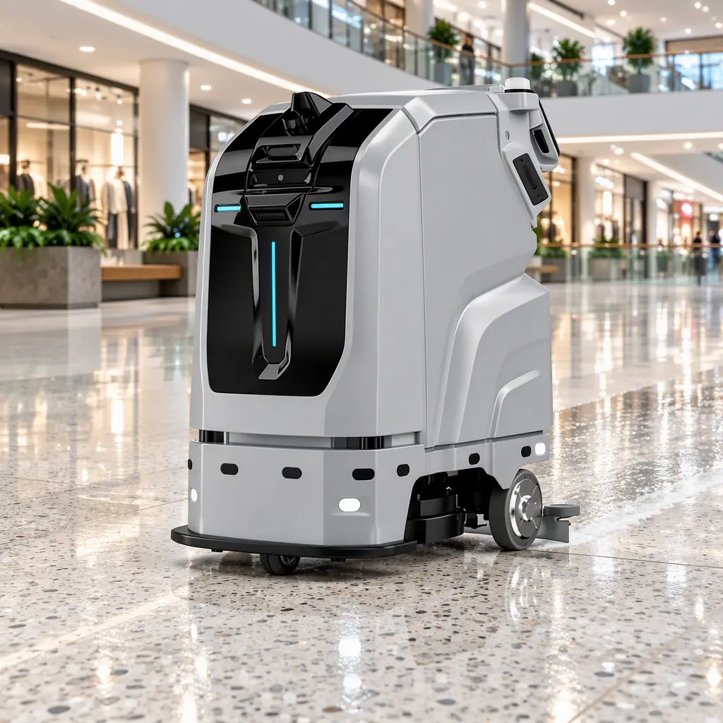
| Machine rated output | 2,040 m²/h | AOMAN C1 published figure |
| Machine availability | 68% | Drains, refills, docks, interventions |
| Effective machine rate | 1,387 m²/h | 2,040 × 0.68 |
| Machine hours per day | 17.3 h | 24,000 ÷ 1,387 |
| Units required | 3 | 17.3 h ÷ 6.5 usable h per unit per day, rounded up |
| Residual labour retained | 30% | 27.7 h/day for detail and daytime work |
| Residual labour cost | USD 242,600/yr | 27.7 × 24 × 365 |
| Gross annual labour saving | USD 565,400/yr | 808,000 − 242,600 |
The gross saving is the number vendors quote. It is not the number that matters. Three cost lines sit between gross saving and real saving, and skipping them is why second-year reviews go badly.
The Three Cost Lines Between Gross and Net Saving
Each of these is computable before purchase, and each is frequently omitted from the seller's model.
| Cost Line | Annual Figure (12,000 m² example) | How It Is Derived |
|---|---|---|
| Consumables and water | USD 14,000–22,000 | Brush and squeegee sets on a 600–900 h replacement cycle, pads, and water at 120 L per tank cycle — far higher than indoor cleaning because debris load drives cycle count |
| Maintenance and support | USD 18,000–30,000 | Preventive schedule through year two onward plus an allowance for unscheduled repairs outside warranty. The structure of this line is set out in the maintenance and TCO guide |
| Fleet operations overhead | USD 25,000–45,000 | Charging energy, dock maintenance, connectivity, software licence, and the supervisor hours spent managing the fleet rather than the crew |
At the midpoint of those ranges the operating cost of the automated case is roughly USD 68,000 per year. Against a gross labour saving of USD 565,400, the net annual benefit lands near USD 497,000 — a figure reduced about 12% from the headline, but still a decisive case.
That 12% is the honest haircut. A model that quotes the gross figure and stops is not a model, and it is the reason some operators report disappointment in year two when the consumable and support invoices arrive.
Payback Arithmetic, and the Assumption That Moves It Most
Payback is capital divided by net annual benefit. The capital side has to include everything required to operate, not just the machines.
| Capital Line | 3-Unit Deployment | Notes |
|---|---|---|
| Machines | Site-specific | Model dependent; AOMAN C1 class specified for large-format mall floors |
| Charging docks | 1 per unit + 1 spare | Docks need a water point and drainage; power planning follows the charging-infrastructure method |
| Commissioning and mapping | One-off | Multi-level sites need per-floor maps plus elevator integration |
| Network and integration | One-off | Multi-floor routes require lift and gateway integration to avoid manual ferrying |
| Staff transition | One-off | Training for retained staff operating the fleet — covered in the staff training guide |
The assumption that moves payback most is not machine price. It is retained labour percentage. Shift that figure from 30% to 50% and the net annual benefit falls by roughly a quarter; shift it to 15% and it rises by more than a third. This is why the pre-purchase task is a task-level labour decomposition — hours by task, not hours by headcount — because the retained figure must be built task by task, not chosen as a round number.
The second most sensitive assumption is cleanable area. A survey that counts gross floor area will inflate the manual baseline, inflate the perceived saving, and produce a model that collapses the first time the finance team asks how the numbers were built.
Where the Model Differs by Building Type
The formula is constant. The inputs are not, and the divergence is large enough that a model built for one building type should never be reused for another.
| Facility Type | Dominant Input Effect | What Changes |
|---|---|---|
| Office tower | Low soil load, high visit frequency | Manual rate is high (300+ m²/h) so the baseline is cheap; savings come from frequency, not depth. Compact 3-in-1 units fit the fixture layout |
| Retail mall | Large open floor, high soil load | Best savings profile for large-format scrubbers; the worked example above is this case |
| Airport or transit hub | 24-hour operation, very large area | Cleaning windows are short and continuous; availability matters more than rated rate |
| Healthcare or laboratory | Compliance-driven procedure time | Manual hours include documented process; the automated case must preserve auditable records |
| Industrial plant | Coarse debris, low frequency | Manual rate drops sharply with debris load; recovery capacity, not sweep width, is the constraint |
| Outdoor and perimeter | Weather-dependent scheduling | Availability falls in wet seasons; the model needs a seasonal curve, not an annual average |
The transit case deserves a note because it inverts a common assumption — the same window-scarcity logic that governs airport and transportation hub deployments. In a 24-hour facility the labour saving often looks smaller per square metre, because the manual baseline is already organised around continuous coverage rather than a shift. The gain there is usually in consistency and in freeing staff for passenger-facing work rather than in raw headcount, and a model that only counts headcount will understate it.
Building the Model for Your Own Site
Six steps, in order, and none of them can be skipped if the output is to survive scrutiny.
- Survey cleanable area, not gross area. Measure room by room and deduct fixed obstructions. This single step is where most models are wrong.
- Measure your manual productive rate. Time a real crew on a real shift including refills and travel. Do not use an industry average.
- Compute the fully loaded labour rate. Base wage plus on-costs plus supervision plus equipment. Ask finance for the figure they use internally.
- Apply a machine availability factor you can defend. Start at 60–70% for a first deployment; operators who have run fleets for a year typically report 70–80%.
- Add the three operating cost lines. Consumables, maintenance, fleet overhead. Ranges above are a starting point, not a quote.
- Model retained labour task by task. List every cleaning task in the building and mark it machine, staff, or both. The hours that remain staff-assigned are your retained figure.
Run the sensitivity on inputs three and six — the labour rate and retained percentage — because those two move payback more than anything else, including machine price. A model that is only tested at one value of each is a forecast, not an analysis. The framework for deciding between purchasing outright and financing the same fleet is set out in the RaaS and financing guide, and the ongoing cost structure that feeds line two above is worked through in the maintenance and TCO guide.
Send us your cleanable area, shift pattern and the split between open floor and detail work, and we will build the model with you — including the sensitivity table, so the case is presented the way finance will examine it. Contact us.