
Service Robot Throughput per Hour and Fleet Sizing
Two Ways to Size a Fleet, and Why Only One Survives Contact With a Building
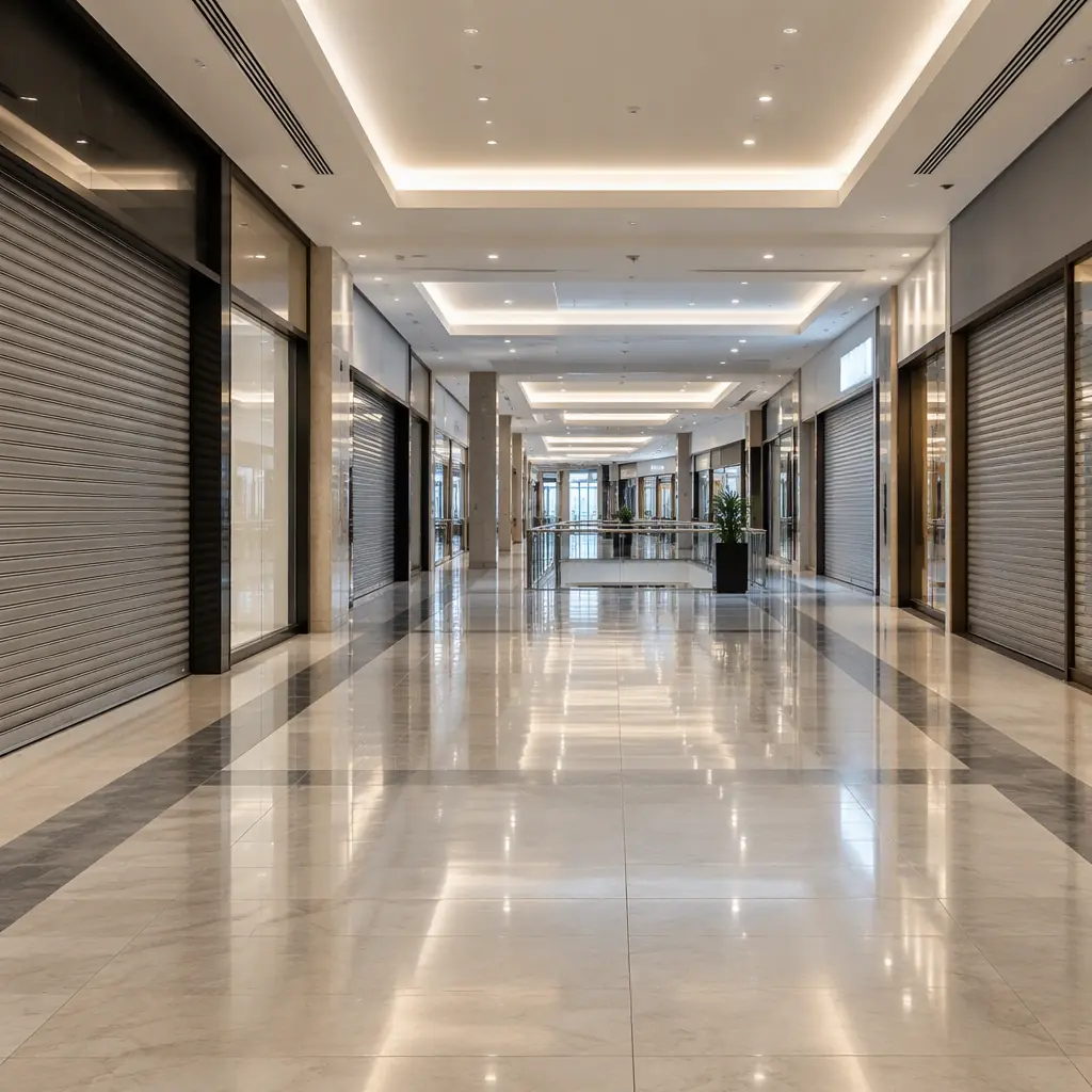
Almost every robot fleet is undersized for the same reason: the unit count is calculated from the machine's headline coverage rate, a figure measured on a clean open floor with a full battery and no obstacles, and then applied to a building full of furniture, lifts, peak-hour traffic and locked doors. The standard published number for a large-format scrubber is in the range of 1,500 to 2,500 square metres per hour. Apply that to a 30,000 square metre shopping centre and the arithmetic gives 12 to 20 hours of work, which looks like one or two machines. In a real building the same fleet usually needs three or four, because the machine does not spend the shift cleaning.
The error is not the vendor's coverage figure, which is honest for what it measures. The error is treating an area rate as an availability rate. A robot working a shift is not cleaning for the whole shift. It is cleaning for the fraction of the shift that remains after transit, dock exchanges, obstacle recovery, blocked-area backtracking, operator intervention and the state-of-charge reserve. Sizing the fleet is the exercise of finding that fraction, and then dividing the real work rate by it.
The Four Numbers That Determine Fleet Size
Fleet sizing collapses to four quantities. Two are properties of the building, one is a property of the machine, one is a property of the operating day. Everything else is derived.
| Quantity | Definition | Typical range | Who controls it |
|---|---|---|---|
| Serviceable area | Floor area actually reachable by the machine on a valid route, excluding stairs, risers, plant rooms and areas behind doors the robot cannot open | 70% to 92% of gross floor area | Building layout and door hardware |
| Field work rate | Measured square metres per hour in production, including overlaps, turns and slow zones | 55% to 75% of the lab coverage figure | Floor finish, layout density, programming |
| Productive fraction | Share of a shift the machine is actually scrubbing | 60% to 78% | Dock placement, transit distance, intervention rate |
| Shift capture | Share of the cleaning requirement that falls inside the operating window the building allows | 50% to 85% | Opening hours and cleaning specification |
Multiplying the first two gives the hourly output honestly attributable to a machine. Dividing that into the required area gives the machine hours the building needs. Dividing the machine hours by the product of the last two gives the machines the building needs. The distinction matters because the first pair is technical and the second pair is operational — and operational factors, not technical ones, are what usually push the unit count up.
The Shift-Capture Problem: Why Night Windows Shrink
Retail and hospitality buildings rarely offer an eight hour cleaning window with the floor empty. A shopping centre that closes at 21:00 and reopens at 09:00 has a twelve hour gap, but the usable portion is smaller than the door times suggest. Security sweeps, deliveries through the service corridor, maintenance access, the fire system test and the early-opening concession staff all consume windows inside it. A realistic analysis often finds six to seven usable hours, not twelve.
That compression interacts badly with a fixed cleaning requirement. If the specification says the food court is scrubbed twice daily and the mall concourse once, the requirement is expressed in passes, not in hours, and the passes have to fit inside the available window. A fleet sized against a twelve hour window and deployed into a seven hour one is undersized by roughly 40 percent, which is precisely the gap that shows up in the first week as an operator manually finishing the overflow zone.
The design response is not always more machines. Three alternatives are usually cheaper, and they should be priced against each other before the order is placed:
- Split the requirement by zone priority. Full coverage in public-facing zones during the window, with secondary zones on an alternating daily pattern. This changes the specification rather than the fleet.
- Use an opportunistic daytime mode. Some scrubbers can work public areas during trading hours at reduced speed with pedestrian avoidance. The rate drops, but the hours available roughly double.
- Move the boundary of the window. A 30 minute extension negotiated with the centre's operations team is often worth more than an extra machine, and costs nothing in capital.
Dock and Transit Overhead: the Hidden 20 Percent
A large-format scrubber with a four hour endurance does not produce four hours of scrubbing. Water capacity, brush wear, filter loading and battery state of charge each impose a practical limit, and the tightest one governs. On a typical 1,200 square metre per hour machine with a 160 litre tank, the tank usually empties before the battery does, at roughly three to three and a half hours of run time.
Every tank exchange costs a fixed overhead: transit to the dock, dump and refill, brush check and transit back. In a building where the dock sits in a service corridor at one end, transit alone can be eight to twelve minutes each way. The arithmetic below shows how quickly that accumulates on an eight hour operating window.
| Parameter | Value |
|---|---|
| Run time per tank | 3.0 h |
| Dock round trip | 18 min |
| Exchange allowance (dump, refill, check) | 7 min |
| Total per exchange | 25 min = 0.42 h |
| Exchanges in an 8 h window | 2 (at 3.0 h and 6.0 h) |
| Overhead consumed | 0.83 h, leaving 7.17 h of available machine time |
| Productive fraction after obstacle recovery (assume 9%) | 6.52 h, or 81% |
Two exchanges look benign in isolation. The problem is that the third exchange — needed if the window is longer than about 9.3 hours — pushes the productive fraction below 75 percent, and a single extra dock positioned at the far end of the building can make the round trip 20 minutes instead of 18. Moving the dock from a remote plant room to a mid-building service closet is a capital cost of a few thousand against a recurring productivity gain of several percent on every shift, for the life of the fleet. It is the highest-return change in most retrofit projects and it is almost never in the original plan. The consumable side of this arithmetic, including water and detergent cost per square metre, is worked through in cleaning robot water and detergent cost.
Work Rate Versus Area Rate: Converting a Benchmark Into a Site Number
The published coverage figure is a lab number under defined conditions. The site number is lower, and the gap is attributable. Four adjustments usually explain it, and each can be measured during a trial rather than guessed.
| Adjustment | Typical effect on the headline figure | How to measure it in a one week trial |
|---|---|---|
| Overlap and edge work | −10% to −18% | Compare total route distance to area covered; overlap is the excess |
| Obstacle density and turns | −8% to −20% | Count interventions and average speed by zone from telemetry |
| Floor finish and soil level | −5% to −15% | Programmed speed will already be reduced on sensitive finishes |
| Doors, lifts and ramps | −5% to −12% on multi-floor sites | Log waiting time at each vertical transition |
A machine rated at 2,000 square metres per hour in the lab commonly delivers 1,300 to 1,500 in a retail concourse and 1,100 to 1,300 in a dense food court with fixed seating. Planning against 1,800 and discovering 1,200 on site is a 50 percent shortfall in capacity, which is the sizing failure that shows up as overtime in month two and as a specification dispute in month six.
Battery Duty Cycle: the Limit Nobody Models First
On a cleaning fleet the binding constraint is usually the tank. On a delivery or patrol fleet it is the battery, and the calculation has a different shape because the work is mission-based rather than area-based.
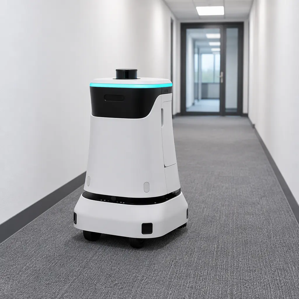
A delivery robot rated for 12 hours of standby may run 6 to 8 hours of continuous delivery, because each mission carries a payload, uses lift cycles and includes empty return legs. A patrol robot on a 20 minute round with a 10 minute dwell at checkpoints spends a meaningful share of its energy on sensors rather than motion. Two rules make the sizing defensible. First, size on a duty cycle that includes the empty return, because return legs typically consume 30 to 45 percent of the energy of a loaded leg and are easy to forget. Second, keep a state-of-charge reserve the machine needs to reach its dock from the furthest point on its route, not from where it usually is. A 20 percent floor computed from an average position is not a reserve; it is an average.
Where charging is the constraint, opportunity charging during natural idle periods changes the arithmetic more than a larger battery does. The dock and charging strategy, and the cost consequences of getting it wrong, are covered in fleet charging infrastructure and power planning. The battery chemistry trade-off between run time, cycle life and cold-weather performance is set out in battery chemistry by duty cycle.
Benchmark Versus Contract: the Expected Throughput Trap
A performance obligation is a fleet sizing decision written in legal language. If the contract sets an availability of 95 percent and defines it as the percentage of scheduled missions started, the vendor is incentivised to schedule fewer missions and the buyer has bought nothing. If it defines throughput in square metres per shift, the buyer has bought capacity, but only if the measurement conditions — area, soil level, window, obstacle density — are the same conditions on which the unit count was based.
The robust approach is to contract on a measured output in a defined window, and to state the exclusion conditions explicitly: closed zones, maintenance windows, construction hoarding, events that occupy the floor. A throughput figure without its conditions is a number that will be argued about in every quarterly review. The definitions that survive audit, and the way to instrument them, are in service robot KPI benchmarks and service credits and availability clauses.
A Sizing Worksheet for the First Order
The sequence below is the one that survives a procurement review. Each line produces a number that can be defended, and each number is measured rather than assumed wherever measurement is possible.
- Start with serviceable area, not gross area. Walk the building and subtract what the route cannot reach. On most sites this alone is a 10 to 25 percent correction.
- Set the field work rate from a trial, or from 60 percent of the lab figure if no trial is possible. Document which.
- Multiply by the productive fraction using the dock round trip you will actually have, not the one you would like.
- Divide the required passes into the result. This gives machine hours per day, which is the number that drives everything else.
- Divide by the usable window, not the door-to-door hours. If the result exceeds the fleet you planned, change the window or the specification before adding units.
- Re-run the whole calculation for the peak day, usually the day after a public holiday or a weekend in a retail site, and size on that day rather than on the average.
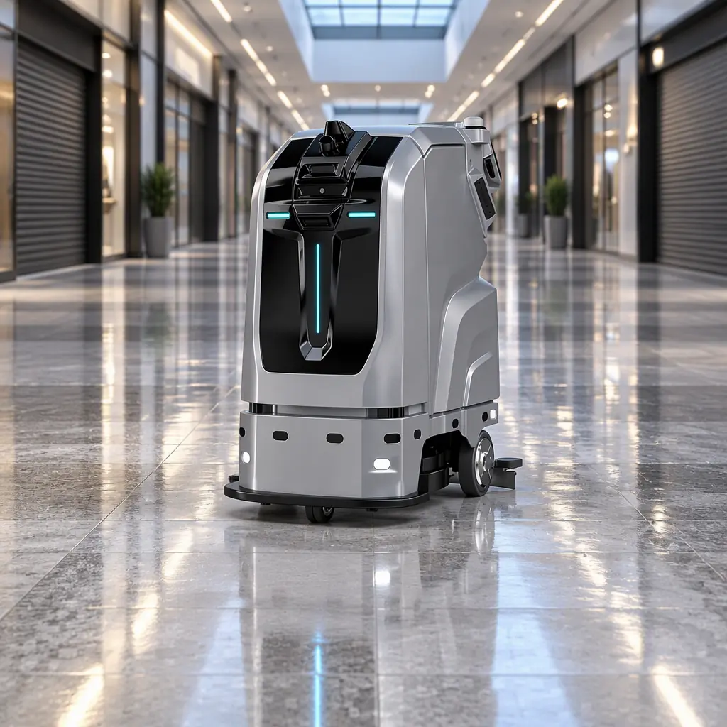
A fleet sized this way will typically be larger than the first estimate and smaller than the operator's instinct, and it will come with a defensible record of why each unit exists. For the machine specifications behind the arithmetic — tank capacity, run time, dock requirement and sensor payload — see the AOMAN C1 scrubber, the AOMAN C2 Pro and the AOMAN D1 delivery robot, or send us your floor plan and we will return a sizing sheet against it.