Service Robot Fleet Demand Charges and Peak-Load Power Economics

Why Kilowatt-Hours Are Only Half the Bill

Commercial and industrial electricity tariffs usually have two main components. The energy charge bills each kilowatt-hour consumed. The demand charge bills the highest rate of consumption sustained in a short interval, typically 15 or 30 minutes, and it is based on the month's peak, not the average. A building that draws 100 kW steadily pays the same demand charge as one that spikes to 100 kW for a single quarter-hour, even though the second consumes far less energy.

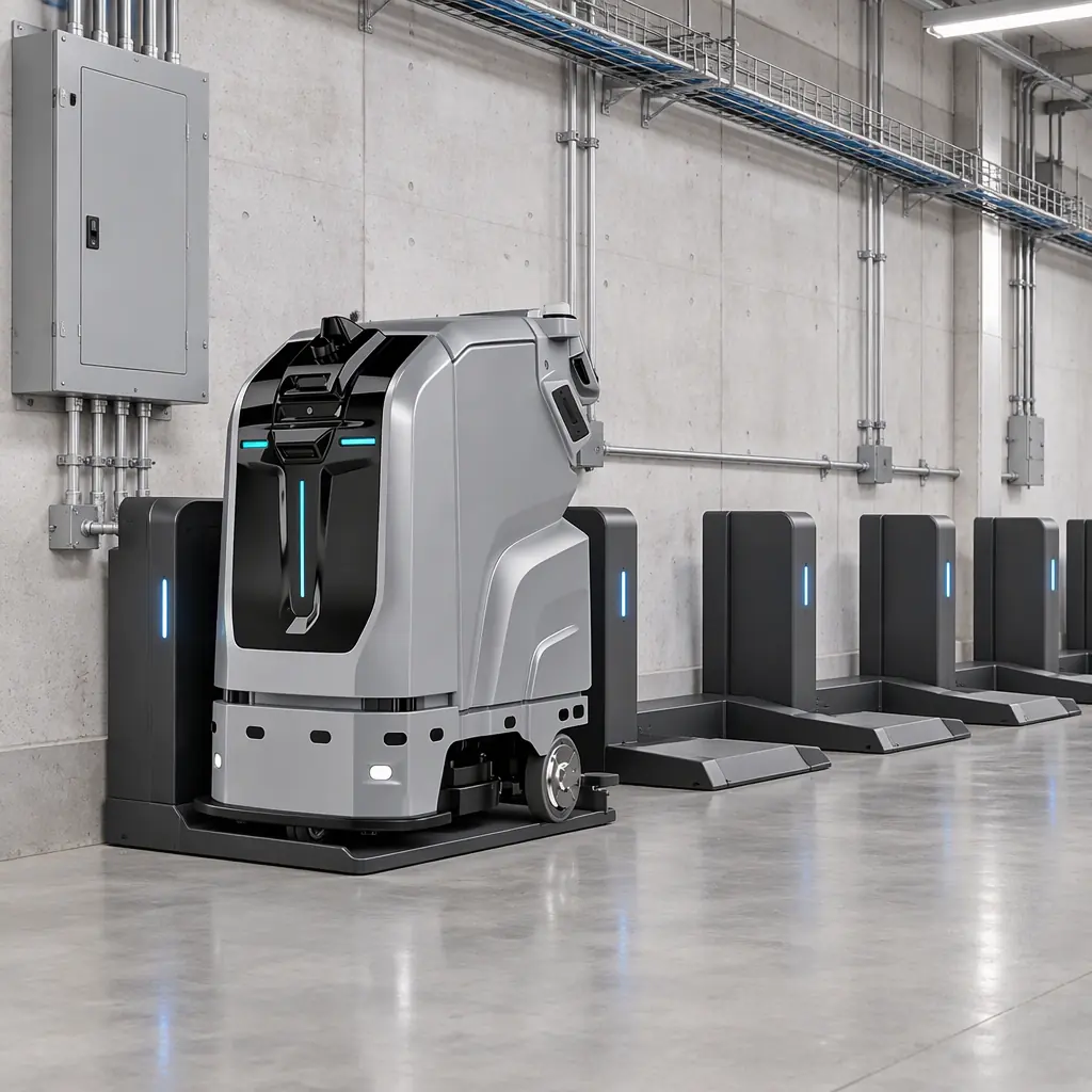
This asymmetry is what makes charging strategy matter. A fleet of scrubbers and delivery units all returning to their docks at shift end and all starting to charge within the same window creates a sharp peak. Halve that peak by staggering the schedule and the demand charge falls with it, even though the total energy is unchanged. The full energy picture, including the load model the scheduling decision rests on, is developed in the charging infrastructure power planning guide, and the narrower per-unit figures are in the electricity cost guide. Demand charges are the layer above both.

Reading a Demand Charge Off Your Own Tariff

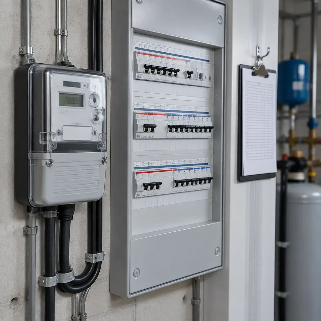
Before modelling anything, find the demand terms in your current bill. They are usually stated in currency per kilowatt, with a separate figure for on-peak and off-peak, and sometimes a ratchet clause that pegs the charge to the highest peak of the last several months. The table below shows the components to identify.

Tariff component	What it looks like on the bill	How a robot fleet affects it
Energy charge	¢ or $ per kWh, often split peak/off-peak	Adds directly; predictable from kWh consumed
Demand charge	$ per kW of monthly peak	Set by the highest 15-30 minute interval; the fleet's charging peak feeds it
Time-of-use bands	Higher per-kWh rate in defined hours	Shifting charging off-peak cuts the energy rate
Ratchet clause	Peak locked to a recent high for months	A single bad peak keeps costing after it passes
Power factor	Penalty below a threshold	Chargers with poor power factor can add a charge

The ratchet is the reason to get this right early. If a poorly scheduled first month sets a high peak that a ratchet holds for a year, the cost is locked in long after the schedule is fixed. Model the charging load before the first unit is commissioned, not after the first bill arrives.

The Load Profile of a Robot Fleet

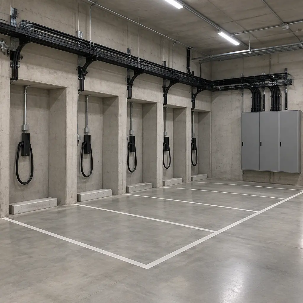
A fleet's draw is not constant, and it is not the sum of every unit's charger rating. It is the sum of what is actually charging at any moment, which depends on duty cycle, battery state, and charger control. The figures below illustrate the shape; substitute your own unit specifications.

Phase	Typical draw per unit	Fleet behaviour
Deep discharge to bulk charge	Near charger rating for the first 30-60 min	This is the peak-creating window
Absorption	Tapering to half or less	Draw falls quickly; the peak is short
Float / maintenance	A few percent of rating	Negligible but continuous
Idle docked, charged	Near zero plus standby electronics	Contributes to base load only
Opportunity charging	Partial top-ups between tasks	Spreads draw, flattens the peak if scheduled

Because the peak comes from the bulk-charge window, the leverage is entirely in when units enter that window. Ten units each drawing 2 kW in bulk phase is a 20 kW peak if they start together, and a 4 kW peak if they are staggered five at a time. The energy consumed is identical; the demand charge is not.

Charger intelligence matters here. Some chargers support scheduled start, current limiting, or load management across a group. If yours do not, a simple timer or a controlled power distribution board can achieve the same staggering. The staging infrastructure that supports this pattern is described in the staging depot and spares planning guide.

Scheduling Moves That Cut the Peak

Reduce the peak with tactics that cost little or nothing to implement. Rank them by effort and take the cheapest first.

• Stagger charge starts. Delay each dock's start by a few minutes so bulk phases do not overlap. This alone removes the sharpest part of the peak.
• Cap simultaneous charging. Allow only a set number of units to bulk-charge at once, holding the rest in a low-draw queue until a slot frees.
• Shift to off-peak. Where the tariff has time-of-use bands, schedule charging into the low-rate window; the energy rate and the demand peak both fall.
• Use opportunity charging. Top up between tasks during low-occupancy periods rather than saving all charging for shift end.
• Sequence by need, not by arrival. Charge the units needed earliest first, and let units with a full shift of margin wait.
• Coordinate with building loads. Avoid charging robots at the same time as HVAC start-up, kitchen equipment, or other large loads that already set the building's peak.

The last point is the one most often missed. The fleet does not need to be the building's largest load to raise its demand charge; it only needs to coincide with whatever load already peaks. Reading the building's load profile and moving robot charging away from the existing peak is often more valuable than any change to the robots themselves.

Building the Cost Model

Turn the tariff and the load profile into a monthly figure. The calculation is straightforward once the terms are known.

1. Energy component. Fleet kWh per month (from the per-unit energy model) multiplied by the applicable per-kWh rate, split by peak and off-peak.
2. Demand component. The highest 15-30 minute interval the fleet adds, in kW, multiplied by the demand rate. Estimate it as the number of units in simultaneous bulk charge times the charger rating.
3. Compare schedules. Compute the demand component for the unstaggered fleet and for the staggered schedule, and take the difference. That difference is the saving the schedule delivers every month.
4. Check the ratchet. Confirm the new peak does not trip a ratchet clause that would lock the higher figure for future months.
5. Fold into TCO. Add the fleet's combined energy and demand cost to the ownership model in the total cost of ownership guide, so the power line reflects the peak and not just the energy.

Modelled this way, demand charges stop being an invisible line on the utility bill and become a design input. A charging schedule is cheap, it improves battery health by avoiding simultaneous thermal load, and it keeps the fleet's power cost proportional to the work it does rather than to the moment it happens to plug in.